Founded in Japan, a Chemical Trading Company (The Company) specializes in plastic and non-plastic products with plastic materials constituting 80% of their sales. Forecast-based sales dominate their sales type, playing a crucial role in aiding companies in managing market fluctuations, inventory planning, and production scheduling. Nevertheless, unforeseen events such as natural disasters or economic downturns can disturb projections, prompting customers to engage in over-forecasting behavior.
Enhancing Sourcing Efficiency through Advanced Analytics: Optimizing Operations with Probability-driven Sales Forecasting
Sale Forecasting Case Study of a Leading Chemical Trading Company
Case Study
Challenge
- The difference in quantities between the forecasting and ordering stages serves as the fundamental reason behind the overstocking situation.
- Increasing Operational Cost: Extra warehouse storing costs (like rent, utilities, insurance), potential write-offs, capital cost of tied-up goods.
- Operational Inefficiencies: Overloaded warehouse space, leading to increased inventory complexity, and packing errors.
ABeam Solution
- Probability analysis on ordering behavior: Detecting over-forecasting behavior and ordering behavior changes based on their provided forecast value range (small vs large quantity of soft order)
- Enhanced Predictive Precision: Optimizing Forecasting Period Selection with Probability Distributions
- Improved decision-making process with scenario analysis
Success Factors
- Gaining a better understanding of customers’ forecast and order behavior.
- Forming the best practices in receiving forecasts and order to reduce the risks of over-forecasting.
- Making purchasing decisions on customer’s actual order derived from historical data.
BUSINESS SUMMARY
PROBLEM OVERVIEW
As a prominent player in the plastic, chemical, and electronics industry, The Company is engaged in the distribution of a diverse range of chemical agents, plastic products, and non-plastic items. The Company is among the first links of complex global supply chains dealing in bulk volumes and greatly sensitive to the bullwhip effect1. To secure the supply, The Company’s customers usually over-forecast, leading to overstocking. The overstocking situation requires opening new warehouses, driving up operational costs, risking write-offs, and tying up capital, thus reducing profitability. In 2022, The Company encountered a significant challenge of excessive stock due to the accumulation of inventory over several years. This overstocking issue amounted to more than 12 million worth of goods. Nearly 7 million USD (US dollars) value of stock ages more than 3 months (standard period), which could reach up to 11 months, surpassing the industry standard.

-
The bullwhip effect refers to a phenomenon in supply chain management where minor fluctuations in customer demand at the retail level result in increasingly significant fluctuations in demand at higher levels of the supply chain, including wholesale, distribution, manufacturing, and raw material suppliers.
We consider a two-stage problem in which the supplier and customer interact as follows.
In the first stage – forecasting stage.
- The buyers provide the supplier with its order forecast (soft order).
- The buyers tend to inflate their orders to secure sufficient supply in volatile markets.
- The supplier commits to the provided forecast of the customer and makes orders with the production source to insure the delivery date for buyer.
In the second stage – actual ordering stage
- The buyers agree to the order but are not forced to order.
- The buyers will (or not) pay a small penalty for any shortfall of its commitment from the forecast.

FORECASTING MODEL CHALLENGE AND SOLUTION
There are some different sources of forecast information which can influence the planning decisions: the demands which are calculated on basis of historical demands realizations, the macro and micro economic factors and the forecasts which are received directly from the customer, i.e., the customer-provided forecasts.
The challenge:
Because of how the chemical industry works, we couldn't use normal factors like prices, marketing, or promotions to better understand our models. Also, the factors that affect demand in this industry are big economic things that are hard to predict. So, we can't use them to guess how much demand there will be in the future.
With traditional time series forecasting, the data also needs to possess certain qualities (continuous and large data points). The intermittent nature of some time series (not continuous demand/order from customers) poses a real challenge in forecasting.
The solution:
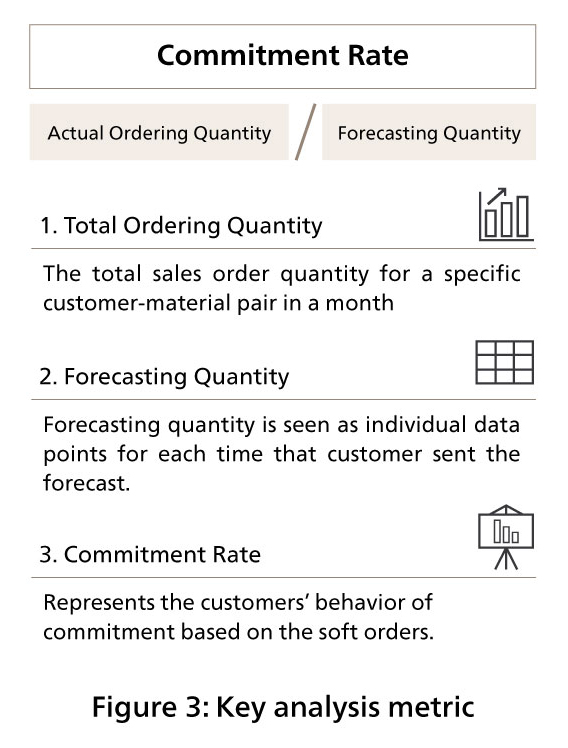
Using the forecast data (soft order) which are received directly from the customer as the signal of the amount of good we need for planning decision; we calculated the commitment rate (as Figure: 3) as a metric for analyzing customer ordering behavior provides valuable insights into their level of actual order behavior.
While time series techniques struggle with the dynamic nature of customer behavior, probability analysis offers better results for forecast-based sales. The probabilistic approach embraces uncertainty by considering soft orders and allows the company to make informed decisions, even when historical patterns are unclear, such as ordering new products or re-ordering after a long time. By acknowledging the unpredictability of customer decisions, probabilistic view equips The Company with a more realistic and flexible forecasting tool, overcoming the limitations of conventional time series methods and providing a range of potential sales outcomes.
The Company can now gain deeper insights into customer preferences and trends through time (Figure 4). We should monitor changes in the probability of customer order behavior over time to adapt our strategies effectively. As customer behavior evolves, probability analysis offers a solid framework for The Company to adjust and improve its predictions, ensuring a more accurate and adaptable forecasting model. This enables us to stay responsive to shifting customer preferences, market dynamics, and external influences, ensuring continued relevance and competitiveness in the marketplace.

PROJECT OVERVIEW
In this case study, we focused on plastic materials, which is the main product of The Company (80% share)
FOUR KEY POINTS IN DESIGNING EFFECTIVE FORECASTING SOLUTION
1.Data Grouping
This refers to the level of detail in your forecast. For example, are you forecasting by products, customers, vendors, or the combination of many factors? The best grouping level will depend on your specific needs and the available data.
The Company needs to consider an accurate forecast at two different grouping levels:
- [Aggregated] Materials x Vendor (~250 combinations) to support vendor ordering planning.
- [Detailed] Materials x Customer (~400 combinations) to optimize pricing and inventory.
The selection of an appropriate data group level for generating forecasts has a direct impact on accuracy of forecasting. In this case study, the problem we want to focus on is the overstocking problem with current high inventory. So, the detailed approach by Materials x Customer is chosen.
2.Temporality
This refers to the forecasting timeframe that aligns with the characteristics of the company’s products and data. This means that we need to focus our attention on a limited forecasting horizon to suit the individual characteristics of each product. To put it simply, we cannot work on three-year-forward forecasts for every single product in the portfolio. Instead, we need to focus our attention on the forecasting horizon that is the most useful.
Example: In considering the case of the production lead time ranging from 2 to 4 months. We should watch out for the forecast data to cover a period of 1 to 5 months before the targeted delivery month.

Orders placed in August, with expected arrivals in October or December, are unlikely to influence inventory levels for the subsequent 2 to 4 months but will have an impact thereafter, particularly from November to January. Additionally, fluctuations in forecasted quantities from customers for the September to January period necessitate a reassessment of order volumes to ensure optimal stock availability.
In short, the best practice is to focus on forecasting demand over the risk-horizon (lead time plus review period) to cover the risks of having too much/too little inventory.
3. Metrics for forecasting evaluation
MAPE (Mean Absolute Percentage Error) is a common metric used to evaluate the accuracy of forecasts. However, it's not always the best choice. MAPE is ideal in the cases where there are little to no outliers, values near zero, values at zero, and low volume or sparse datasets. Other metrics might be more appropriate depending on the specific needs. For example, MAE (Mean Absolute Error) provides protection against outliers, whereas RMSE (Root Mean Square Error) provides the assurance to get an unbiased forecast.
In this case study, the dataset exhibits numerous outliers, marked by sudden and significantly high forecasts from customers. This anomaly has led to a skewed forecast. Consequently, we have opted to employ the Mean Absolute Error (MAE) as the key performance indicator (KPI) for our forecasting analysis.
4. Decision making with model results
Forecasting helps businesses in many ways. While relying solely on data analytics can lead to missed opportunities, a balance between data analytics and intuition can provide a comprehensive view for decision making. Effective forecasting strategies incorporating with them can help businesses reach their desired goals, maximize their resources, and lead to increased profits and long-term success.
Within this project, we not only deploy a forecasting model but also simulate many scenarios based on the assumptions related to the inventory policy and risk tolerance of The Company. Business users can harness their expertise alongside the insights derived from the forecasting results to gain a deeper understanding of their customers' behavior.
RESULTS
Comparison on two scenarios of forecasting results

In the optimistic scenario
With a broader confidence level, The Company may accept more orders, signaling readiness to handle increased volume or variety.
Reduce 55% overstocked quantity, compared to overstocks may occur with original forecasting from customer.
In the conservative scenario
Narrower confidence level: the company opts for a reduced ordering quantity to mitigate the risk of overstocking.
Reduce 85% overstocked quantity, compared to overstocks may occur with original forecasting from customers.
ROI CALCULATION & IMPLEMENTATION ROADMAP
Basically, this solution can break even after 13 months (including 04 months of execution period).

HOW THE COMPANY LEVERAGES DATA SCIENCE
THE COMPANY integrates data science into its operations with five advanced analytics solutions: Predictive Sales Forecasting Model, Selling Price Calculation Tool, Incoming Goods Allocation Tool, Truck Allocation Tool, and Inventory Management Dashboard. The focus showcased in this case study is the Predictive Sales Forecasting Model, where data are analyzed to anticipate future sales accurately.

Customer Profile
- Business Activities
- Industry Chemical Trading Company
- Product
-
- Plastic, chemical and electronics business
- Medical devices
- Food & Beverages
- Dosimetry Laboratory Service
- Detection capability of energies of OSL - Qulxel type
Apr 12, 2024
- Corporate data and titles are those in use at the time of writing.
Click here for inquiries and consultations